WGCNA文献学习与配置
WGCNA文献和hdWGCNA文献阅读
WGCNA介绍
研究背景
Weighted correlation network analysis (WGCNA)是一种系统生物学方法,用于描述bulk RNA-seq中基因之间的相关性模式。WGCNA可用于寻找高度相关基因的聚类(module),使用模块的特征基因或模块内hub基因对基因聚类情况进行汇总,将模块相互关联并与外部样本性状(使用特征基因网络方法)相关联,计算模块隶属度指标(模块与性状的关联)。该方法为基于网络的基因筛选方法提供了便利,可用于识别候选生物标志物或治疗靶点。这些方法已成功应用于多种生物背景,如癌症、小鼠遗传学、酵母遗传学、脑成像数据分析等。WGCNA R软件包是R函数的综合集合,包括网络构建、模块检测、基因选择、拓扑性质计算、数据模拟、可视化以及与外部软件接口等功能。
流程图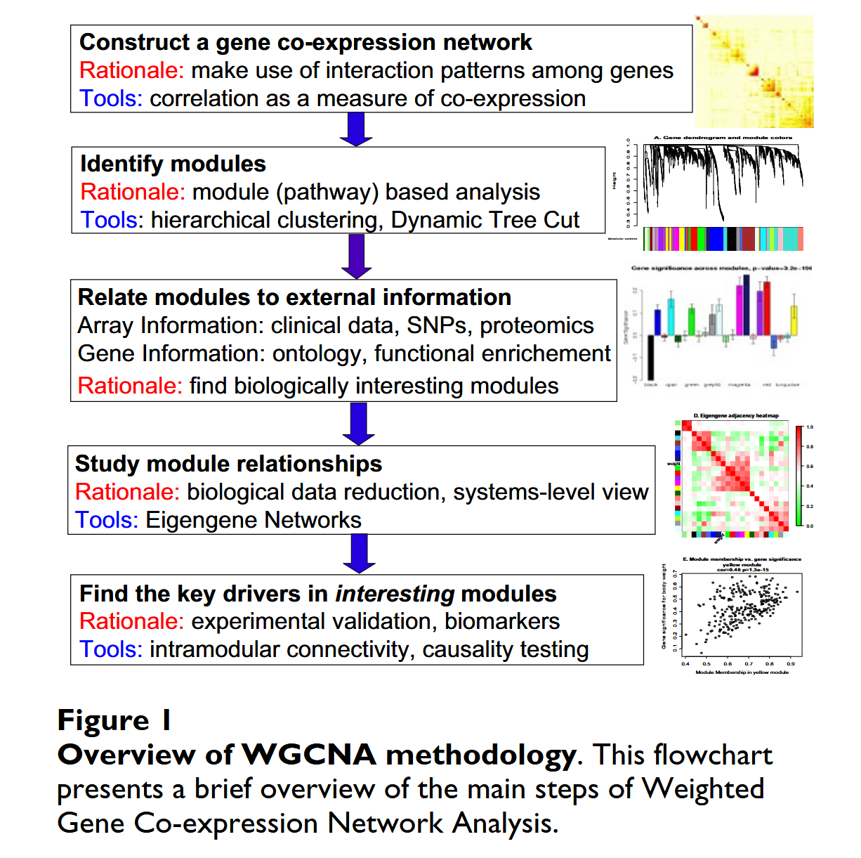
- 构建基因共表达矩阵网络:计算基因间相关性
- 基于Spearman method计算基因的相关性矩阵(Similarity Matrix)
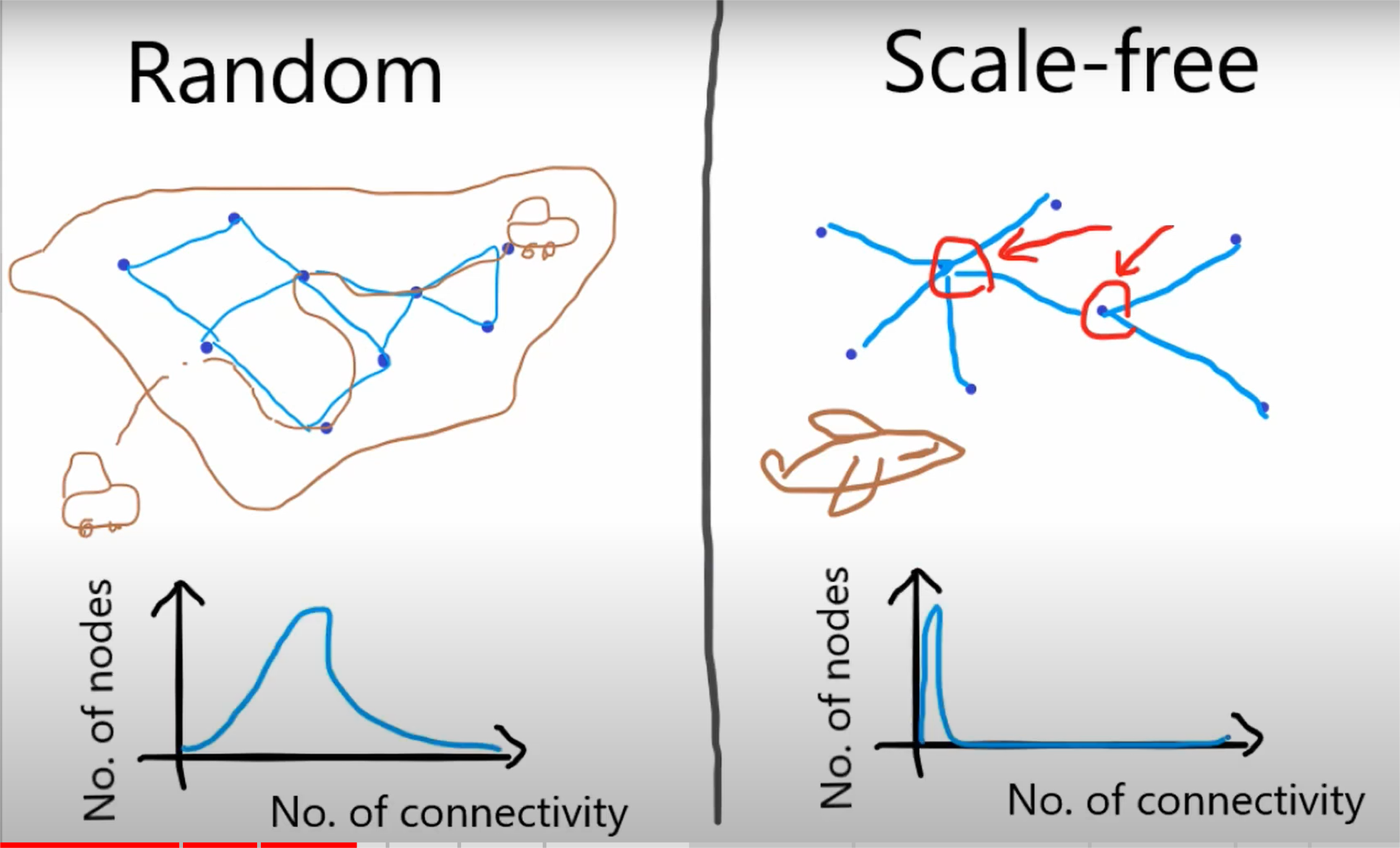
- 将相关性矩阵转化为邻接矩阵(Adjacency Matrix);Similarity Matrix被认为是undirected, weighted gene network,因此从Similarity Matrix转换到Adjacency Matrix的过程,被认为是从无向加权网络转移到scale-free network的过程。
- 此步骤需要选择网络的类型(官方更推荐Signed或者Signed hybrid)
- Unsigned: Genes are similar if they are strongly correlated
- Signed: Only applied to genes that are similar if they are positively correlated
- Signed hybrid: Negative associations are all treated as zero. (与signed network类似,与Signed network的差异可以很小)
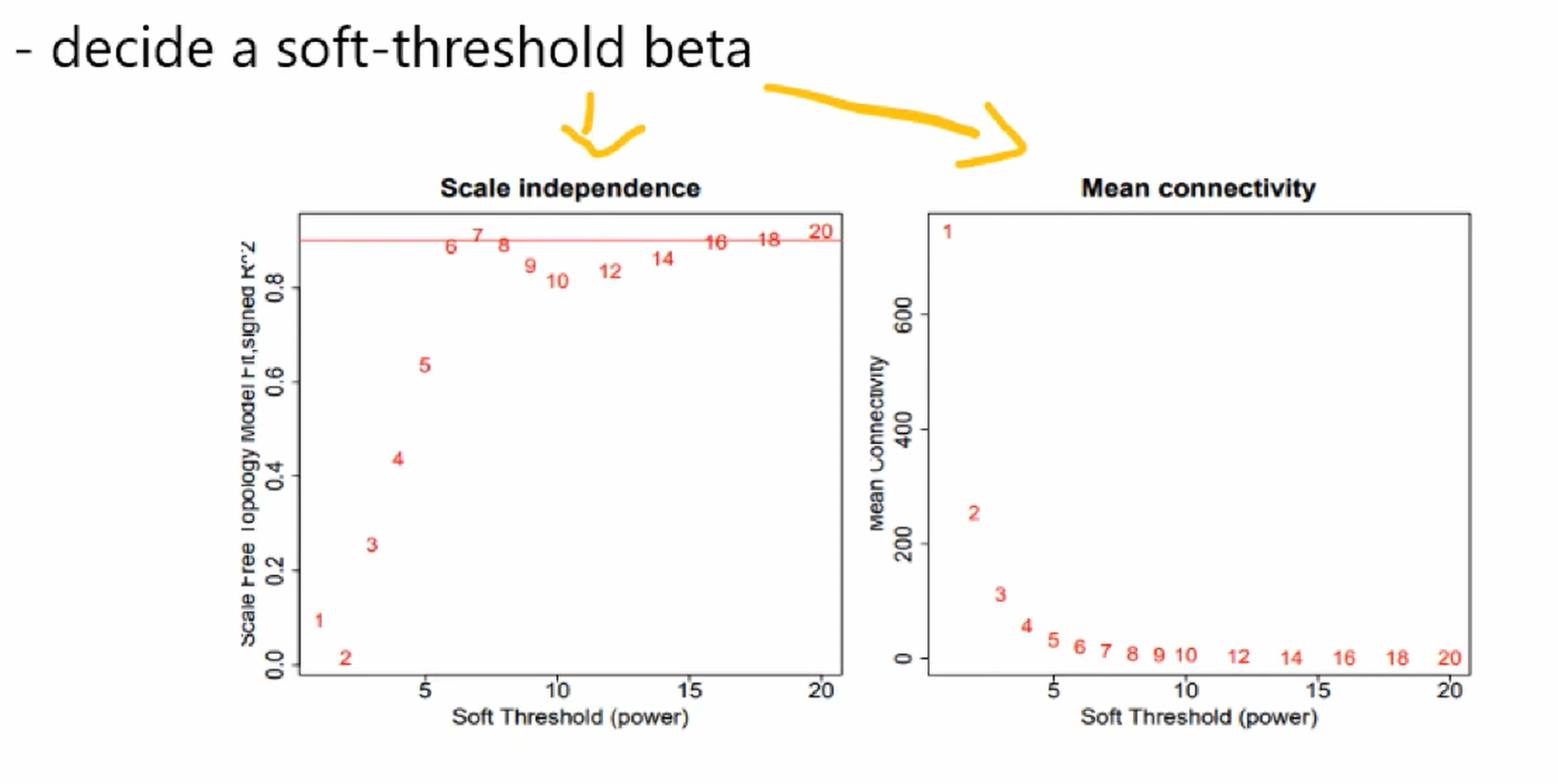
- 根据两个标准,选择soft thresholding β值 (Power selected);soft thresholding β值用于将Similarity Matrix转换到Adjacency Matrix
- Scale independence, 该图的点的纵坐标越高,越接近scale free network。
- Mean Connectivity;由于在scale free network中,大多数节点的连通性较差,因此平均连通性越低,越接近scale free network。
- 此步骤需要选择网络的类型(官方更推荐Signed或者Signed hybrid)
- 根据Adjacency Matrix绘制TOM plot (topological overlap matrix)
- 基因网络的拓扑重叠热图(Heatmap plot of topological overlap in the gene network)是对基因相似性的评估。
- 在热图中,每一行和每一列对应一个基因,浅色表示低拓扑重叠,渐变深的红色表示高拓扑重叠。如果基因在网络中与相似的一组基因相连,那么它们被认为具有高度的拓扑重叠。
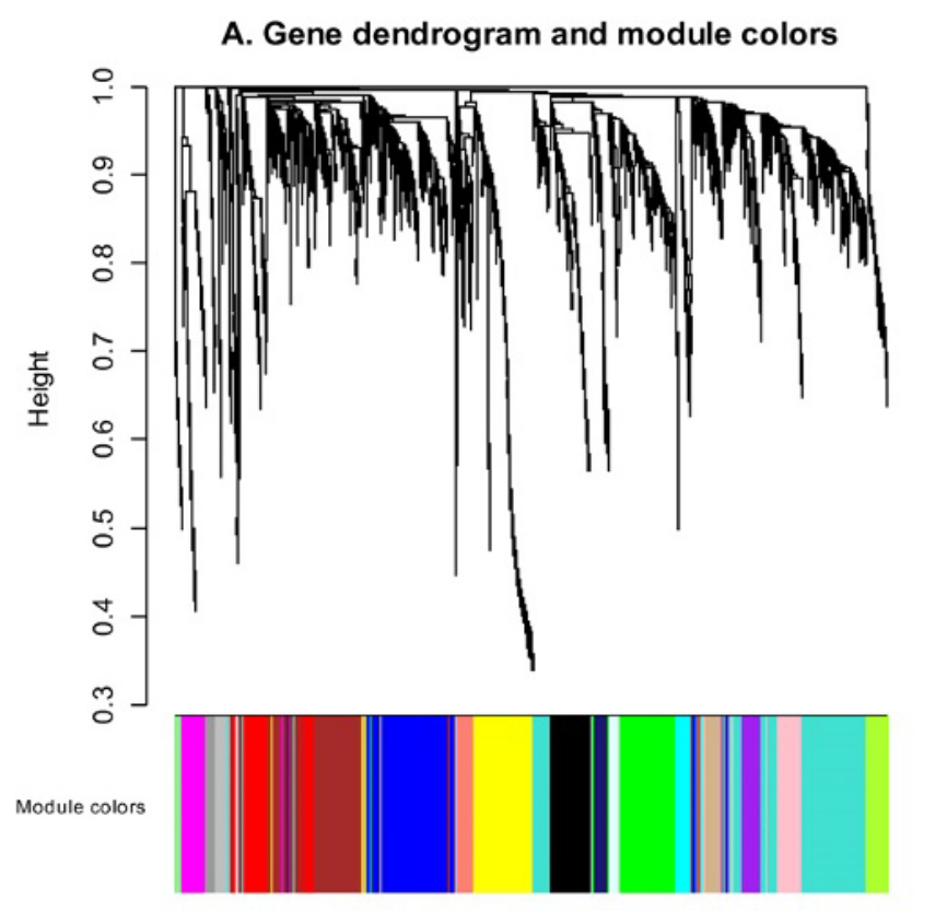
- 模块寻找:基于矩阵的数值进行成对比较,进行层次聚类,并通过Dynamic tree cut对聚类树进行模块划分
- 模块的特征向量值signed module eigengene (ME),反映了节点在模块内的隶属度。然后对特征基因高度相关的模块进行合并。
- 模块的特征向量值signed module eigengene (ME),反映了节点在模块内的隶属度。然后对特征基因高度相关的模块进行合并。
- 将模块与表型相关联:寻找有生物学意义的模块
- 具有高性状显著性的模块可能代表与样本性状相关的通路。
- 模块间相关性研究(Optional)
- 寻找模块内部的key drivers(Optional)
Tips:
Scale-free network 可轻易从无标度网络中寻找到hub genes(The highest-degree nodes)
官方建议删除Counts很低的基因(例如,删除所有在 90% 以上的样本中计数小于 10 的基因),因为这种低表达的Feature往往反映噪声,且基于计数的相关性大多为零并没有真正意义。实际阈值应基于实验设计、测序深度和样本计数。
无论是使用 RPKM、FPKM 还是简单的归一化计数,只要所有样本都以相同的方式处理,对 WGCNA 分析并没有太大影响。
hdWGCNA
1. 初始化配置
注:在SetupForWGCNA步骤后,不建议对seurat对象进行subset(因为subset后WGCNA的输入基因可能无法代表原始的seurat对象)
gene_select参数的三种模式,选择不同的WGCNA输入基因:
variable: 使用Seurat对象中的高变基因
fraction: 使用在整个数据集或每组细胞中特定部分细胞中表达的基因,使用group.by指定。(在Demo中,我们将选择在这个数据集中至少5%的细胞中表达的基因。)
custom: 使用自定义列表中指定的基因。
1 | |
2. 构建metacells
初始化配置后,需要从单细胞数据集构造构建metacells(元细胞)。
由于counts矩阵的稀疏性,会导致较大的方差,导致单细胞数据直接计算Pearson基因相关性会不准确。解决这个问题的一种方法是使用metacells的方法。
简单来说,元细胞是源自同一sampleid的小群相似细胞的聚集体。使用k近邻(KNN)算法找到 K 个最近邻居,识别相似细胞,并将它们进行聚合,然后计算这些细胞的平均或总表达,从而产生元细胞基因表达矩阵,使用元细胞的基因表达矩阵进行下游分析(分析思路类似细胞metadata矩阵,含有对细胞的分类信息等)。与Counts矩阵相比,元细胞表达矩阵的稀疏性大大降低,并提供了对转录状态更稳健的估计。因为像WGCNA等的相关网络方法对数据稀疏性很敏感,使用元细胞作为此类分析技术的输入会更稳健、噪音更小;且在处理大数据(例如分析数百万个单个细胞)时要分析的细胞数量减少(约 100 倍)。很多单细胞表观基因组方法,如Cicero,在构建共可及性网络之前采用了类似的元细胞聚集方法。
可参考:Tommy的blog
函数MetacellsByGroups,用于构建元细胞表达矩阵。该函数为元细胞数据集构建一个新的Seurat对象,该对象存储在hdWGCNA实验内部。该group.by参数确定将在哪些group中构造元细胞。我们只想从来自相同生物样本的细胞中构建元细胞,因此通过group.by将该信息传递给hdWGCNA至关重要。此外,我们通常为每种细胞类型分别构建元细胞。因此,在Demo中,我们按Sample和celltype进行分组,以获得期望的结果。
要聚合的单元格的数量k应该根据输入数据集的大小进行调整,通常较小的k可以用于小数据集。通常使用20到75之间的k值。Demo使用k=25。元细胞之间允许的重叠细胞数量可以使用max shared参数进行调整。(这里的参数可以根据细胞数量调整k值)
注:当存在细胞数极少的细胞类型(由于极端细胞数导致代表性差的细胞类型)时,按照group.by=celltype进行构建metacells的hdWGCNA表现不佳。例如,在Demo数据集中,脑血管细胞是细胞数最少的celltype,我们已经从这个分析中排除了它们。MetacellsByGroups有一个参数min cells,用于排除小于指定cell的group。如果最小cell的值过低,可能会出现错误。
hdWGCNA将group.by中所有输入的参数进行组合,形成新的metacell_grouping列,并要求每个metacell_grouping内的细胞数大于min_cells(默认值100),否则会被过滤掉。
K值的设置: kNN k值越小,方差越大,偏差越小,k值越大,偏差越大,方差越小。k的选择很大程度上取决于输入数据,因为具有更多异常值或噪声的数据可能在k值较高时表现更好。建议k值设置为奇数。hdWGCNA推荐使用20到75之间的k值。
1 | |
Tips: 参数ident.group会改变seurat_obj@misc$tutorial$wgcna_metacell_obj@active.ident的分组信息。seurat_obj@misc$tutorial$wgcna_metacell_obj是构建好metacells后的metadata信息,参数group.by会改变metadata的行名,若输入多个group.by参数,比如c(“cell_type”, “Sample”)会使得行名(细胞barcodes)变为”cell_type1#Sample1_1”,”cell_type1#Sample1_2”这种格式。
group.by输入的参数必须包含ident.group的输入。
3. 共表达网络分析
3.1 配置表达矩阵
这里我们指定用于网络分析的表达式矩阵。因为我们只想包含抑制性神经元这群细胞,所以我们必须在构建网络之前对表达数据进行取子集。hdWGCNA包括SetDatExpr函数,用于存储将用于下游网络分析的一组给定细胞的转置表达矩阵。默认情况下使用元细胞表达矩阵(使用metacells=TRUE),但hdWGCNA确实允许在需要时使用单细胞表达矩阵。该函数允许用户指定从哪个data slot获取表达式矩阵,例如,如果用户希望应用SCTransform而不是NormalizeData的矩阵。
1 | |
同时对多个细胞类型或clusters执行共表达网络分析,需要向group_name参数传入字符向量。
1 | |
3.2 soft-Power(软阈值)设置
WGCNA将相关性矩阵转化为邻接矩阵(给相关性进行幂次计算,使得基因间的连通性符合幂率分布规律)。选择合适的软阈值以减少相关矩阵中存在的噪声量,从而保留强连接并去除弱连接。
函数TestSoftPowers执行不同软阈值的参数扫描。该函数通过对不同power值的网络拓扑情况进行检查,帮助我们在构建共表达网络时指导选择软实力阈值。共同表达网络应该具有无标度的拓扑结构,因此TestSoftPowers函数对不同软阈值下共表达网络与无标度图的相似程度进行建模。此外,我们还包含了一个函数PlotSoftPowers来可视化参数扫描的结果。
此步骤的networkType的参数设置和图像输出与WGCNA相似。
1 | |
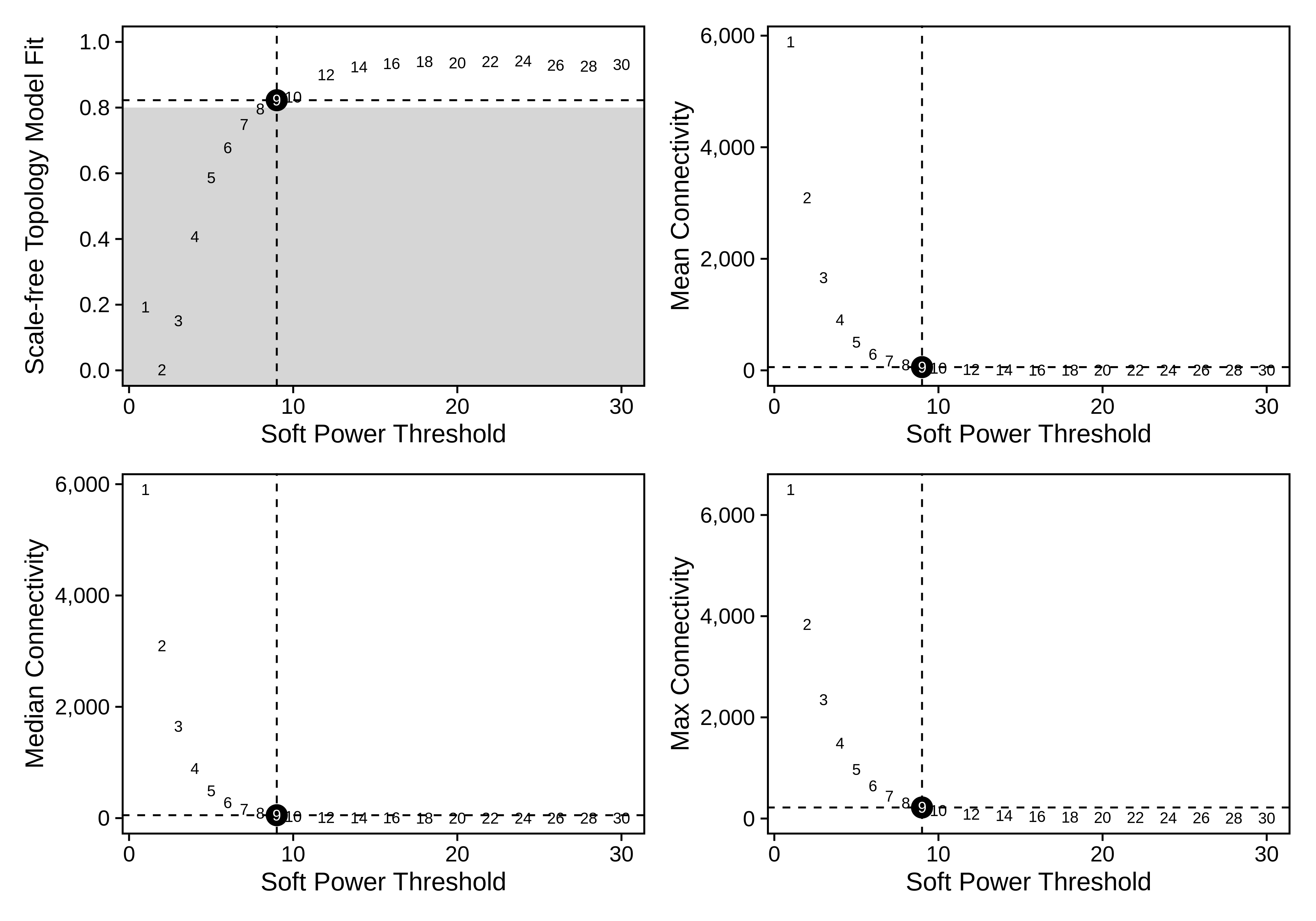
- Scale independence, 该图的点的纵坐标越高,越接近scale free network。纵坐标需要大于等于 0.8 才认为该网络是无标度拓扑模型。
- Mean Connectivity, Median Connectivity, Max Connectivity: 由于在scale free network中,大多数节点的连通性较差,因此这三个指标越低,越接近scale free network。
如果用户没有提供软阈值,则ConstructNetwork将自动选择软阈值。软阈值参数扫描的输出表可以使用GetPowerTable函数查看
1 | |
3.3 构建共表达网络
使用hdWGCNA函数ConstructNetwork,它在底层调用WGCNA包的blockwiseConsensusModules函数。blockwiseConsensusModules的参数可以用相同的参数名直接传递给ConstructNetwork。下面的代码使用上面选择的软阈值来构建共表达网络。
1 | |
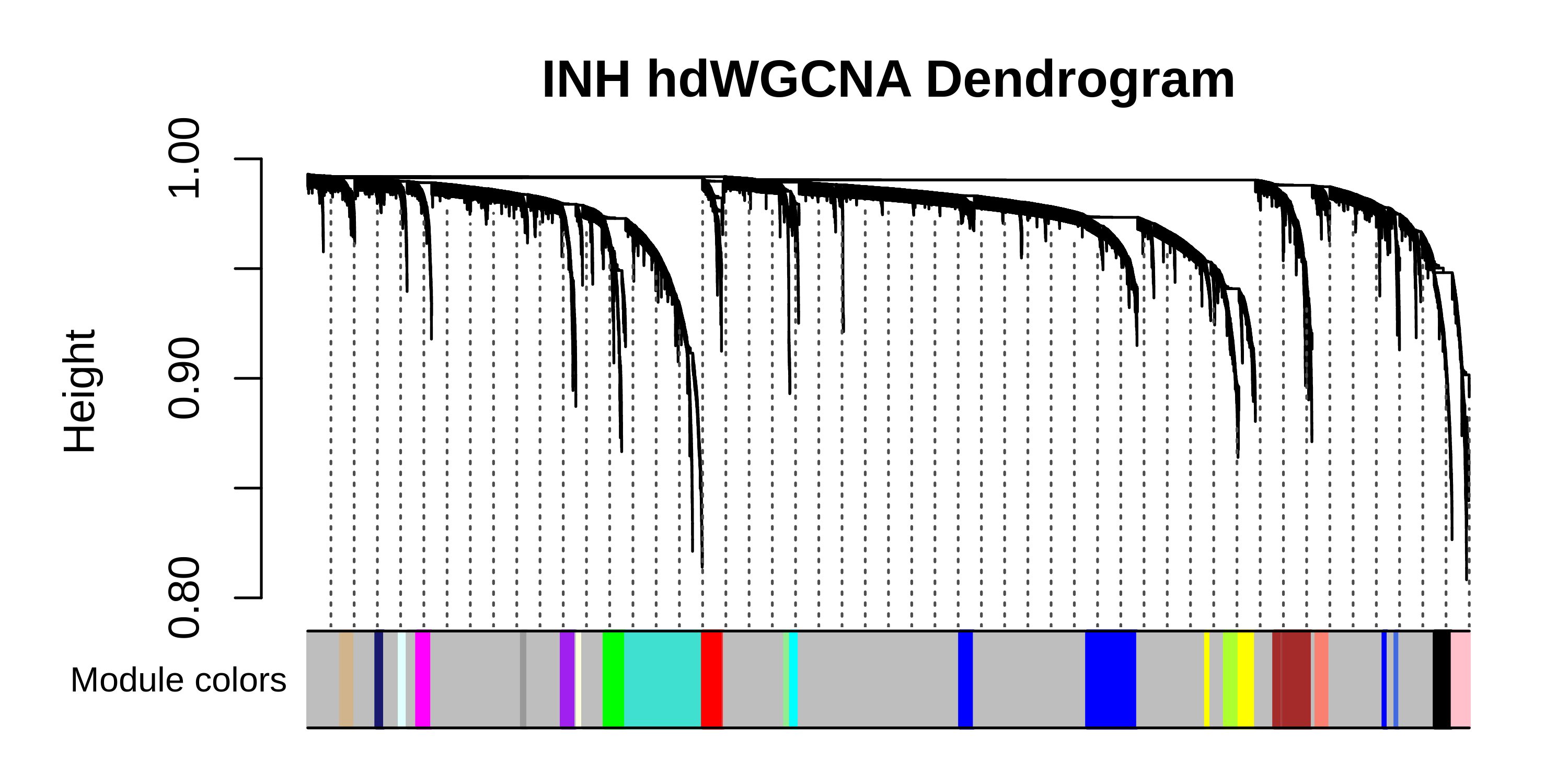
函数plotdendprogram用于可视化WGCNA树状图,该图用于显示由网络分析产生的不同共表达模块。树状图上的每片叶子代表一个基因,底部的颜色表示共表达模块分配。与WGCNA相同,灰色模块由不属于任何共表达模块的基因组成。对于所有下游分析和解释,应该忽略灰色模块。
1 | |
3.4 topoligcal overlap matrix (TOM) 图
hdWGCNA将共表达网络表示为topoligcal overlap matrix (TOM)。这是一个基因对基因的方阵,其中每个值都是基因之间的拓扑重叠。当运行ConstructNetwork时,TOM被写入seurat对象,我们可以使用GetTOM函数将其加载到R中。高级用户可能希望检查TOM以进行自定义下游分析。
1 | |
4. 模块特征基因与连通性
4.1 计算模块特征基因
Module Eigengenes (MEs,模块特征基因)是一种用于度量整个共表达模块的基因表达谱的方式。简而言之,通过对包含每个模块的基因表达矩阵的子集执行(PCA)来计算模块特征基因。每个PCA矩阵的第一个PC是MEs。直观地说,它是一个“被合成的基因”,它是该模块中所有基因的最佳代表。
函数ModuleEigengenes用于计算单个细胞中的模块特征基因。此外,我们允许用户对MEs应用Harmony批量校正,从而产生harmonized module eigengenes(hMEs)。下面的代码使用group.by.vars参数执行由基于Sampleid进行Harmony的模块特征基因计算。
1 | |
ME矩阵存储为矩阵,其中每行是一个细胞,每列是一个模块。可以使用GetMEs函数从Seurat对象中提取该矩阵,该函数在默认检索hMEs。
1 | |
4.2 计算连通性
在共表达网络分析中,我们通常希望关注hub-gene,即在每个模块中连通性最高的基因。因此,我们希望确定每个基因的基于MEs的连通性,也称为kME。hdWGCNA使用ModuleConnectivity函数来计算完整的单细胞数据集中的kME值,而不是元细胞数据集。
这个函数本质上计算基因和模块特征基因之间的两两相关性。可以为数据集中的所有细胞计算kME,但我们建议在运行ConstructNetwork后的celltype或group中计算kME。
1 | |
可以根据模块具体的生物学意义对模块进行重命名。
模块重命名说明书
1 | |
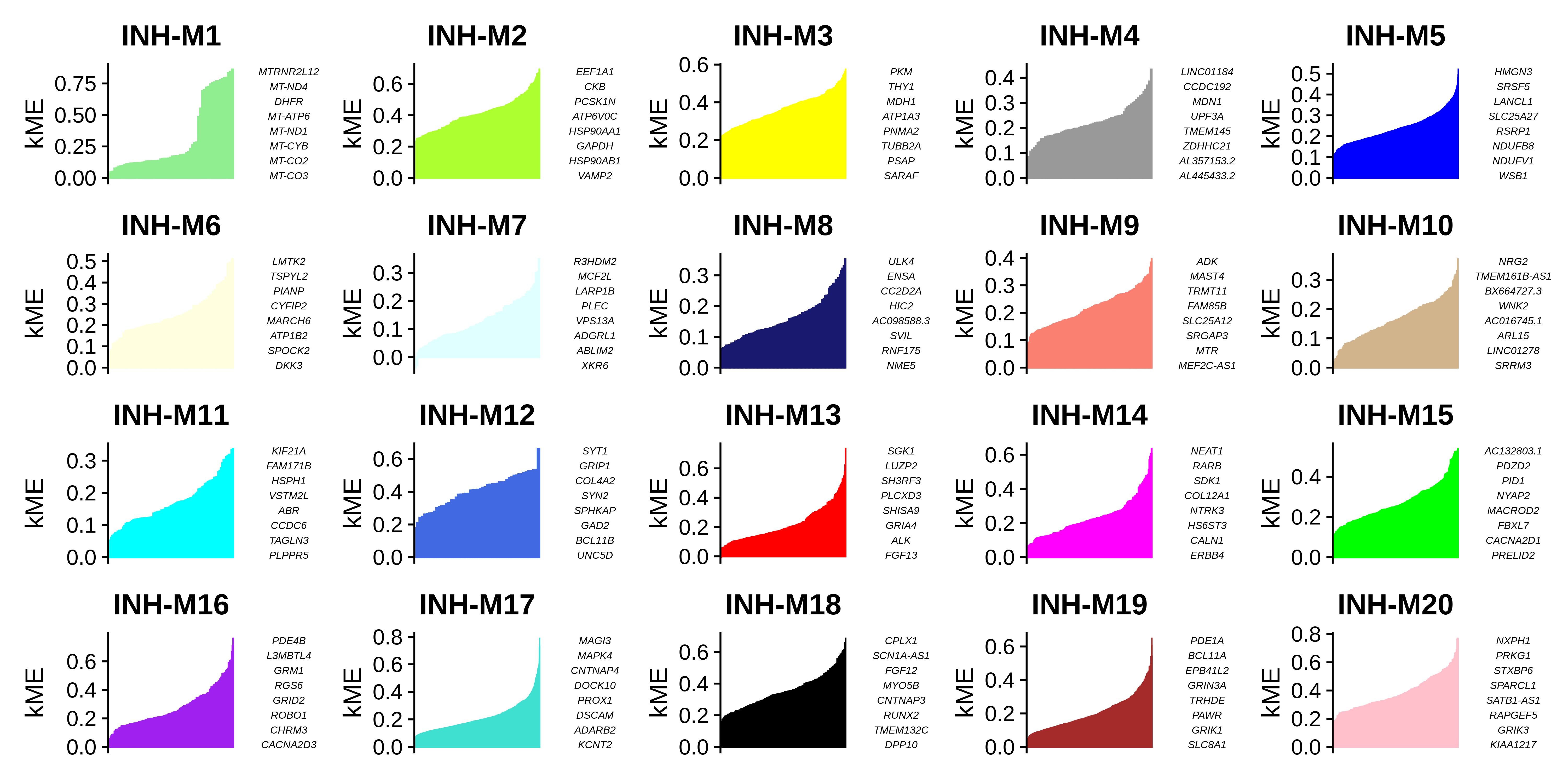
我们可以使用PlotKMEs函数可视化每个模块中按kME排序的基因。
1 | |
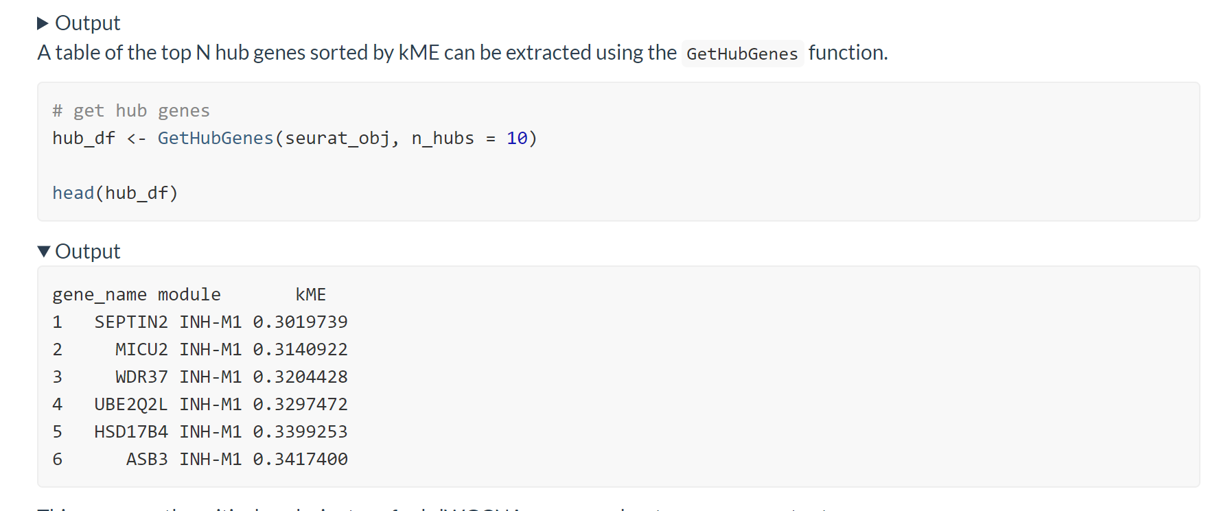
4.3 获取模块分配表
hdWGCNA允许使用GetModules函数轻松访问模块分配表。
该表由三列组成:geneID,存储该基因的模块,模块颜色,这在许多下游绘图步骤中使用。如果调用ModuleConnectivity函数,则会为模块分配表添加额外的kME列。
1 | |
到此为止是hdWGCNA的主体分析流程,记得保存结果。
1 | |
4.4 计算hub-gene打分
Gene scoring是单细胞转录组学中一种常见的方法,用于计算一组基因的总体特征得分。Seurat使用AddModuleScore函数进行打分,但也有其他方法,如UCell。hdWGCNA使用ModuleExprScore函数,用于计算每个模块给定数量的基因的基因分数,基于Seurat或UCell算法。基因评分是通过计算模块特征基因来展示模块表达情况的另一种方法。
1 | |
5. 使用Seurat进行基础的下游可视化
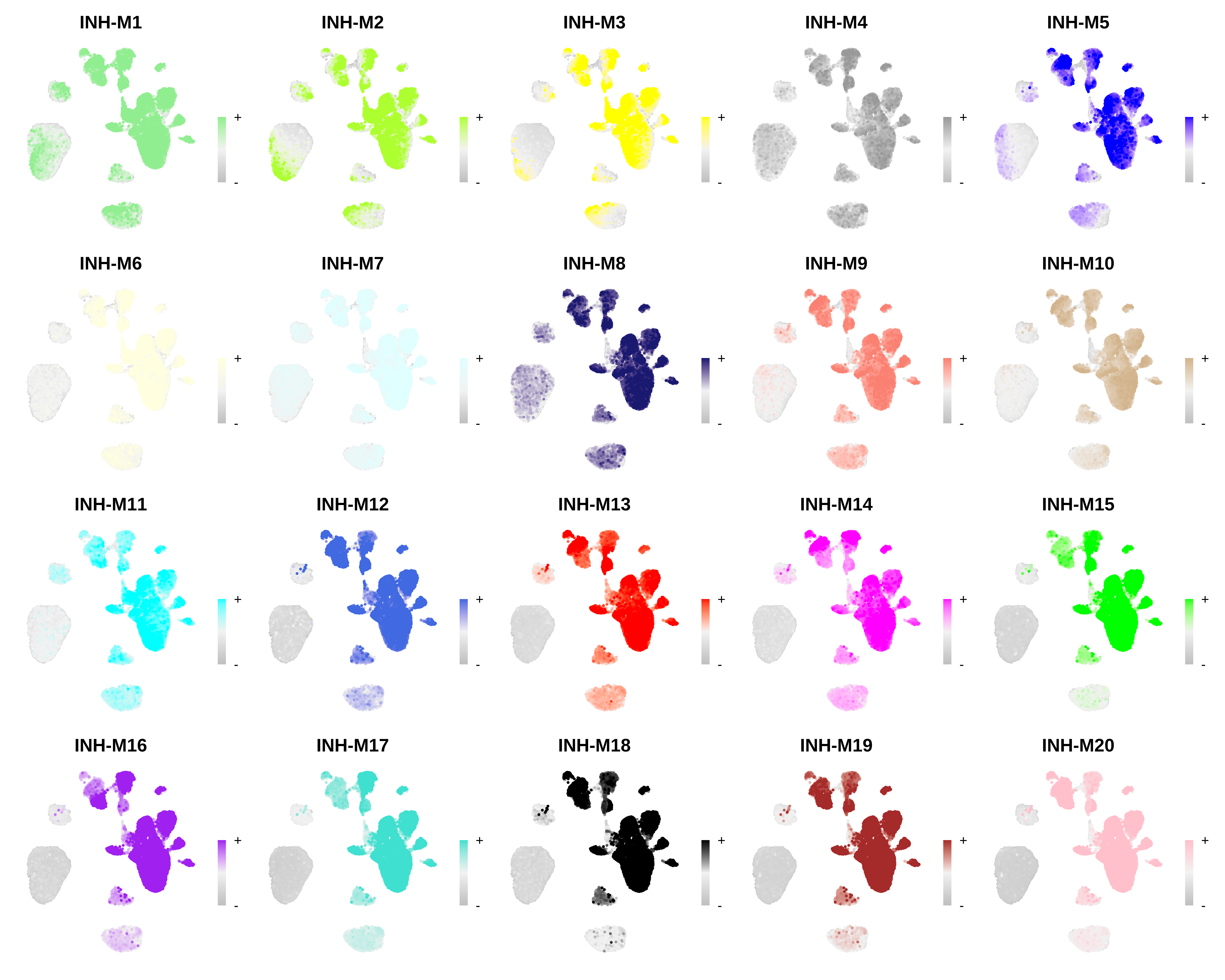
Featureplot
ModuleFeaturePlot函数,用于为每个共表达模块构建由每个模块指定的唯一颜色着色的featureplot
1 | |
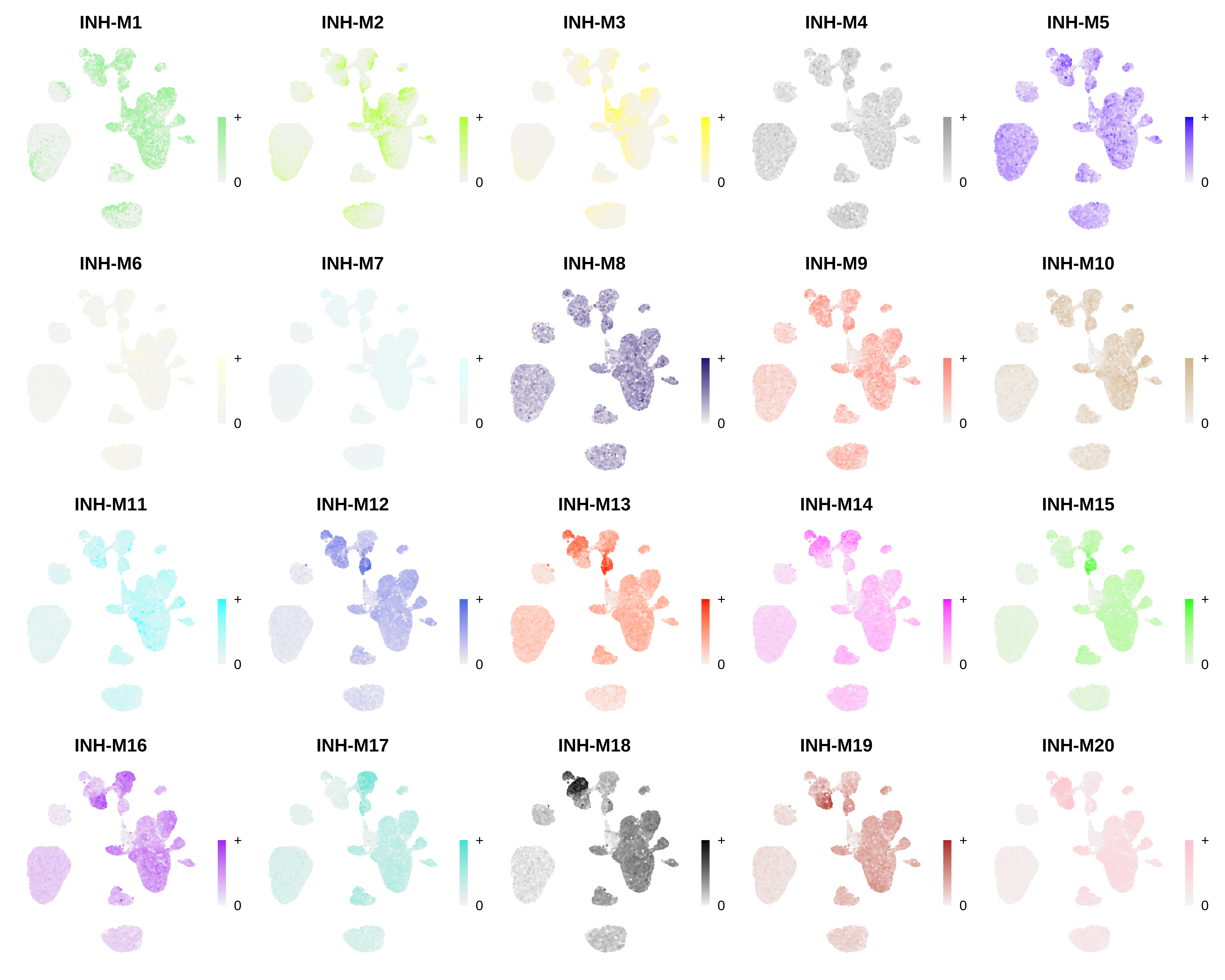
可以使用相同的函数绘制hub-gene的打分情况
1 | |
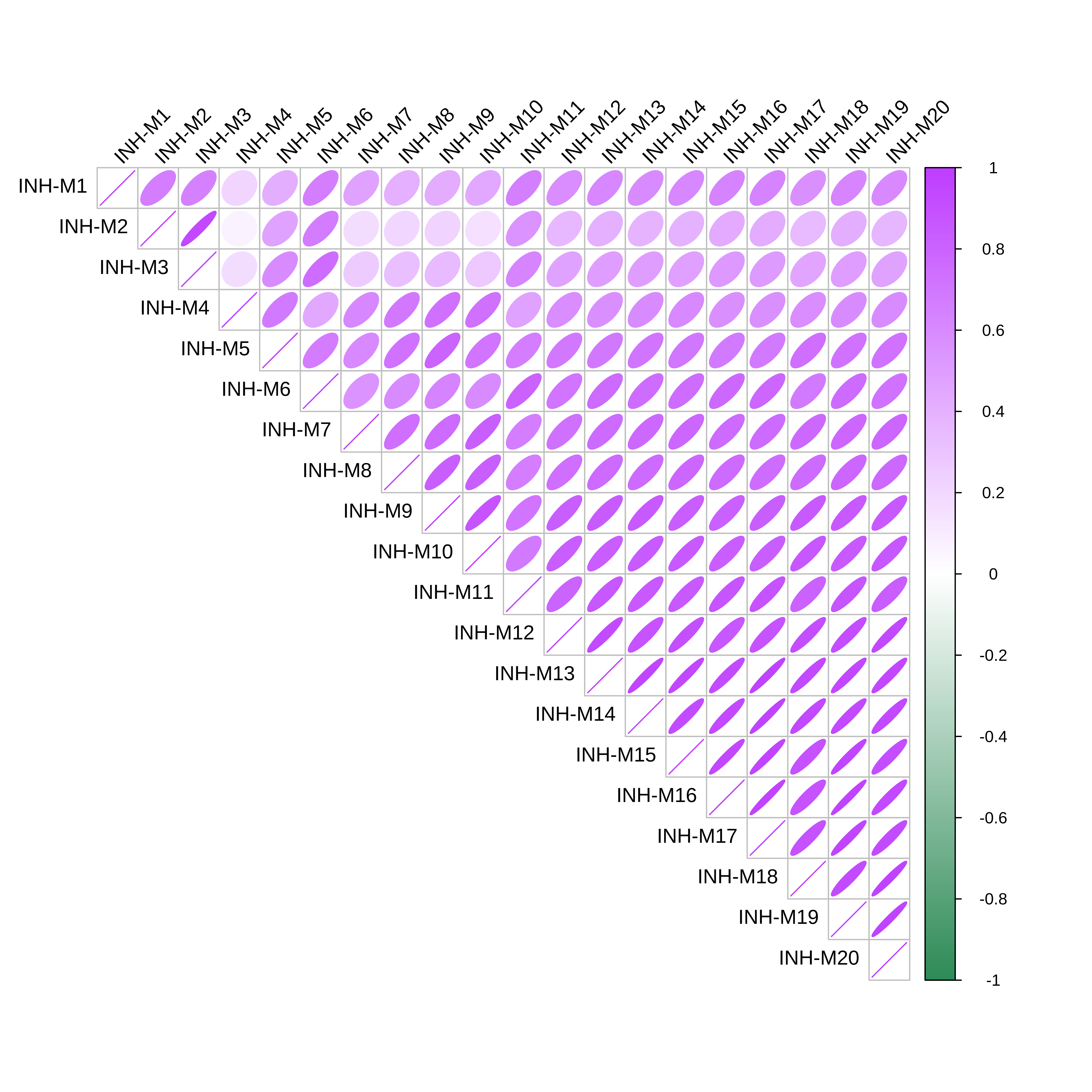
模块相关性
ModuleCorrelogram函数,可以使用R包corrplot根据每个模块的hMEs, MEs或hub基因评分来可视化每个模块之间的相关性。函数默认使用的是hMEs。
1 | |
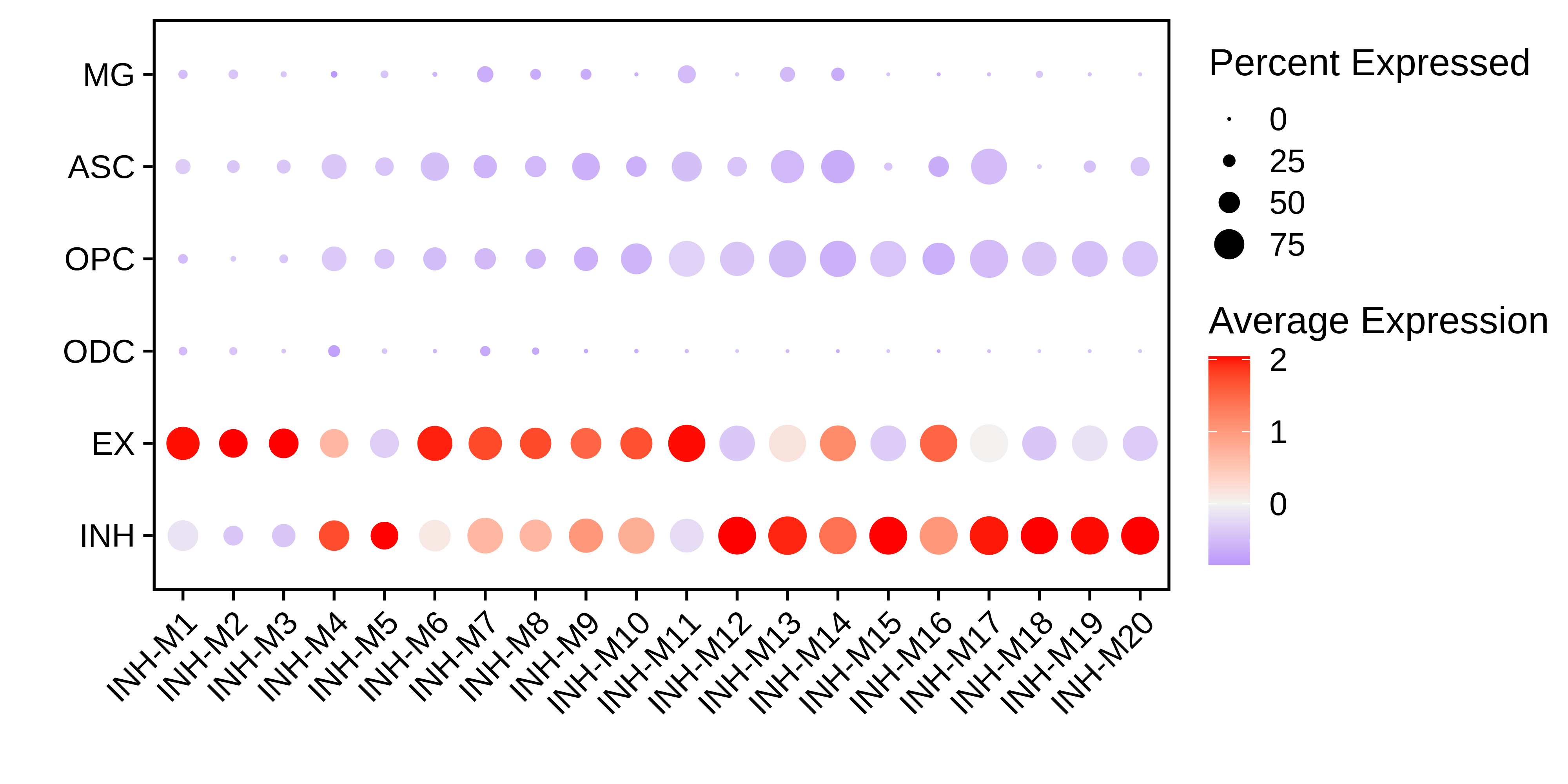
DotPlot
将hMEs数据添加到metadata中进行绘制
1 | |
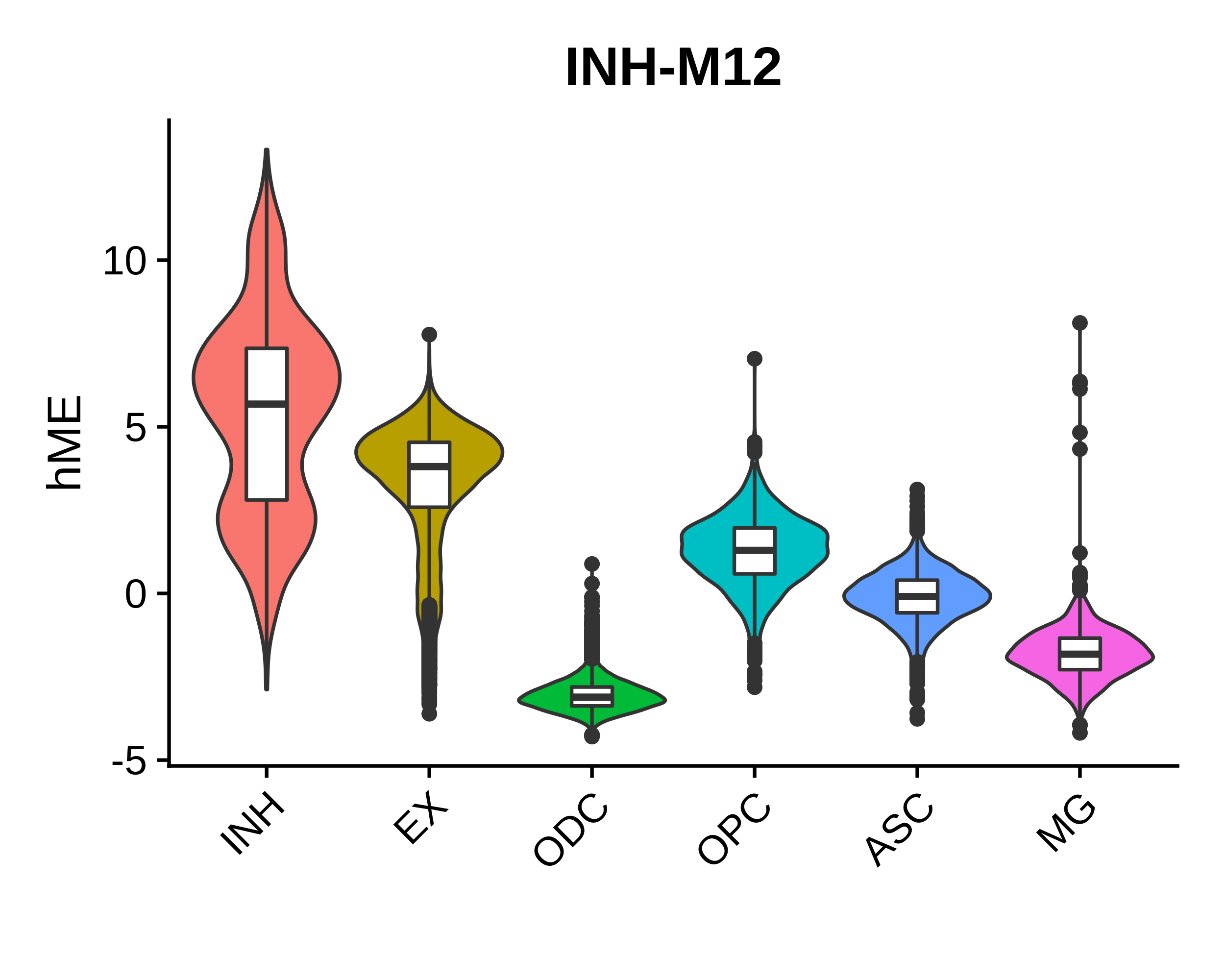
Vlnplot
1 | |
6. 网络分析
加载环境
1 | |
为每个模块生成单独的网络图
ModuleNetworkPlot显示每个模块的单独网络图,按kME显示前25个基因。
1 | |
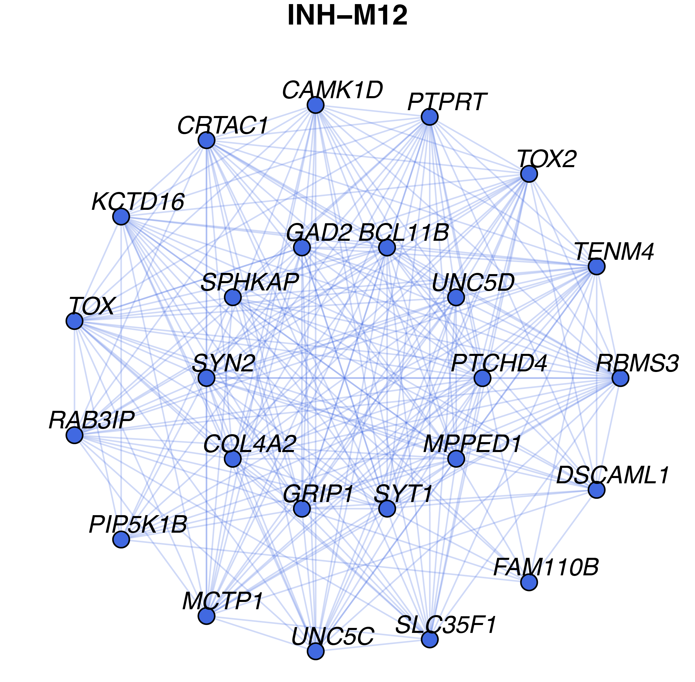
在该网络中,每个节点代表一个基因,每条边代表网络中两个基因的共表达关系。每个模块网络图都是根据hdWGCNA模块分配表GetModules(seurat obj)中的颜色列进行着色的。kME排名前10位的枢纽基因位于图的中心,其余15个基因位于外圈。
可调节参数美化图片:
- edge.alpha:确定网络边缘的不透明度
- vertex.size:确定节点的大小
- vertex.label.cex:确定基因标签的字体尺寸
可视化由每个模块给定数量的hub-gens组成的网络
HubGeneNetworkPlot可视化由每个模块给定数量的中心基因的所有模块组成的网络。该函数取用户指定的前n个枢纽基因和其他随机选择的基因,采用force-directed graph drawing algorithm 力导向布局算法构建一个联合网络。
为了视觉清晰度,可以使用edge prop参数对网络中的边的数量进行下采样。在下面的例子中,我们将每个模块的前3个hub-gene和其他6个基因可视化。
1 | |
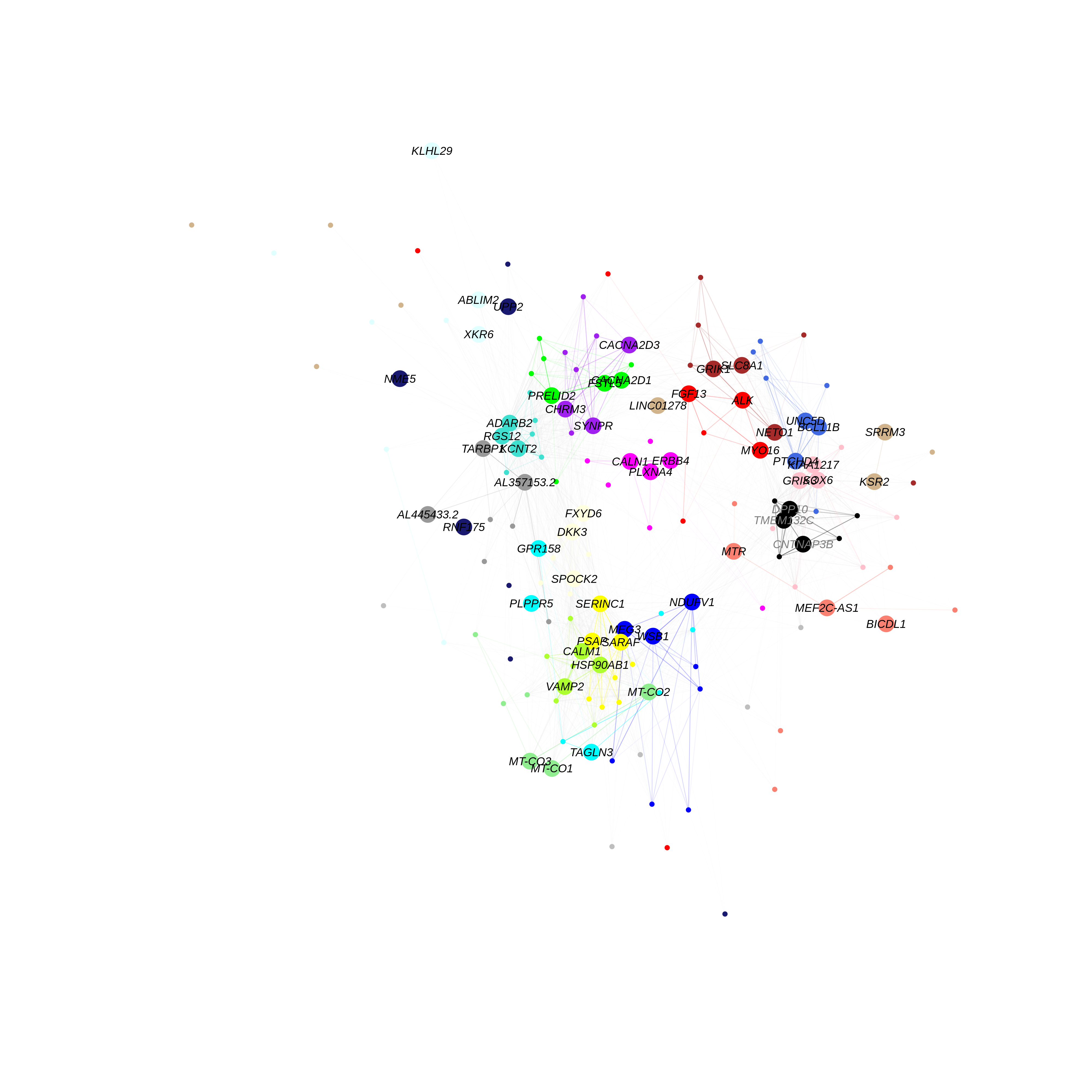
每个节点代表一个基因,每个边代表一个共表达关系。在该网络中,我们用模块的颜色对模块内的边上色,对模块间的边上色。该网络中边缘的不透明度由共表达关系的强度来定义。附加的网络布局设置可以传递给图中layout_with_fr函数。用户还可以通过指定return graph = TRUE来返回要绘图的igraph对象。
g <- HubGeneNetworkPlot(seurat_obj, return_graph=TRUE)
使用Umap同时可视化共表达中的所有基因
ModuleUMAPPlot函数使用UMAP降维算法同时可视化共表达中的所有基因。
hdWGCNA包含RunModuleUMAP函数,基于TOM矩阵运行UMAP算法。对于UMAP分析,我们将TOM中的列子集设置为仅包含每个模块按kME排列的前n个中心基因,n由用户指定。因此,每个基因在UMAP空间中的位置取决于该基因与hub-gene的连通性。该函数利用了uwot R包中的UMAP实现,因此uwot:: UMAP函数的附加UMAP参数(如min dist或spread)可以在RunModuleUMAP中使用。
1 | |

在这个图中,每个点代表一个基因。每个点的大小按其指定模块的基因的kME进行缩放。可以使用ModuleUMAPPlot函数来绘制基因及其共表达关系,并可视化模块UMAP中的基因(但并未可视化底层网络。)
1 | |
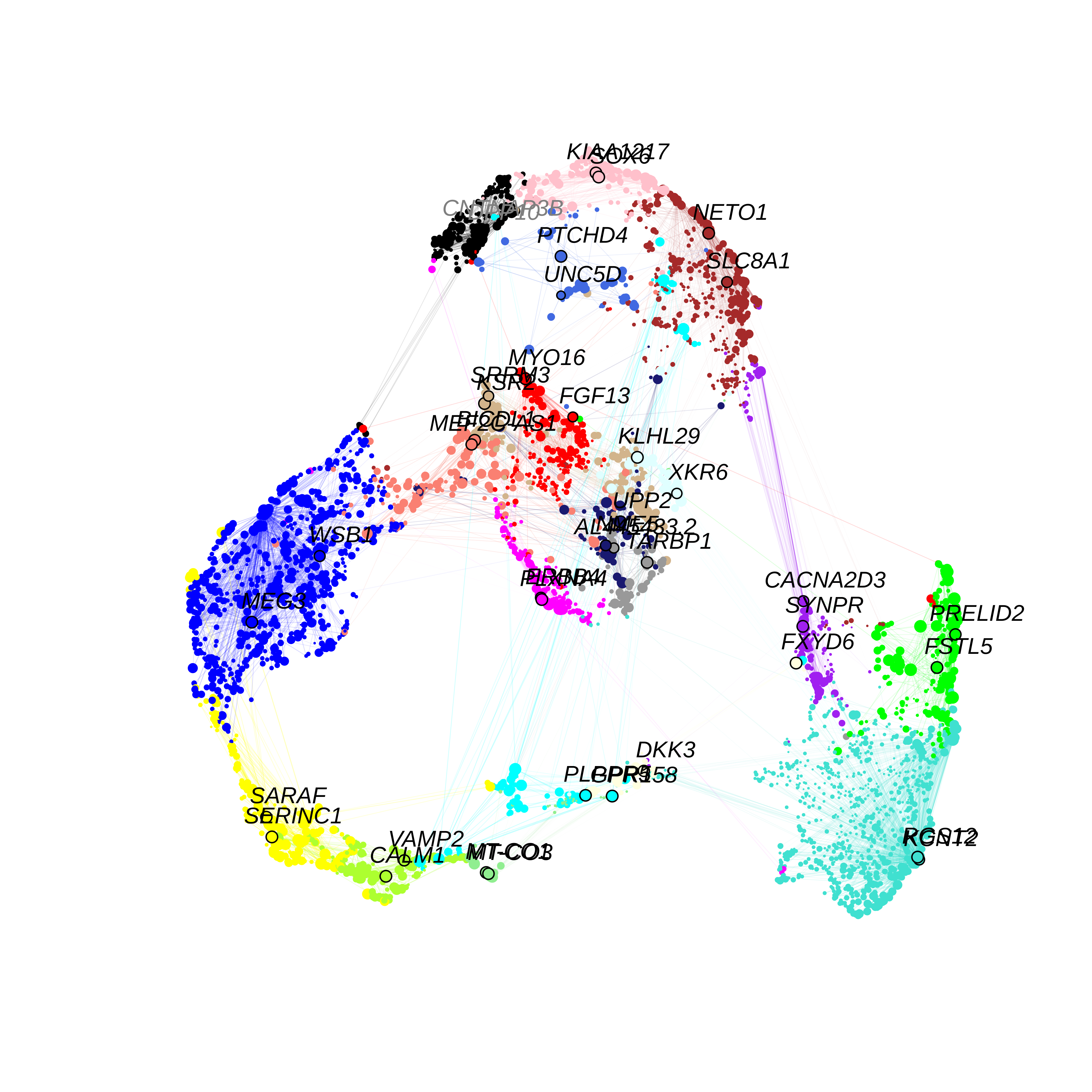
这张图与我们用ggplot2绘制的图相似,但我们展示了共表达网络,并在每个模块中标记了2个hub-gene。为了视觉清晰度,我们使用edge prop参数下采样,只保留该网络中20%的边。我们还允许用户返回igraph对象来制作他们自己的自定义图或执行下游网络分析.
1 | |
可视化改变hub-gene的数量对uamp的影响
我们在UMAP计算中包含的hub-gene的数量会影响下游可视化。在这里,我们使用gganimate来直观地比较用不同数量的hub-gene计算的umap。
1 | |
有监督的Umap,略
7. Differential module eigengene (DME) analysis
执行差异模块特征基因(DME)分析,揭示在给定group中上调或下调的模块。
首先加载环境
1 | |
两组比较
这里我们讨论如何在两个不同的组之间执行DME测试。使用hdWGCNA函数FindDMEs,这是Seurat函数FindMarkers的一个特例。使用Wilcoxon test,来比较两组,但其他test可以通过test.use参数调用。
由于教程数据集只包含对照大脑样本,我们将使用性别来定义我们的两个group。FindDMEs需要group1和group2的barcodes列表。此外,我们将只比较来自INH clusters的细胞,因为我们对INH clusters执行了网络分析。
首先获取group1和group2的barcodes列表
1 | |
执行FindDMEs
1 | |
使用函数PlotDMEsLollipop对结果可视化
1 | |
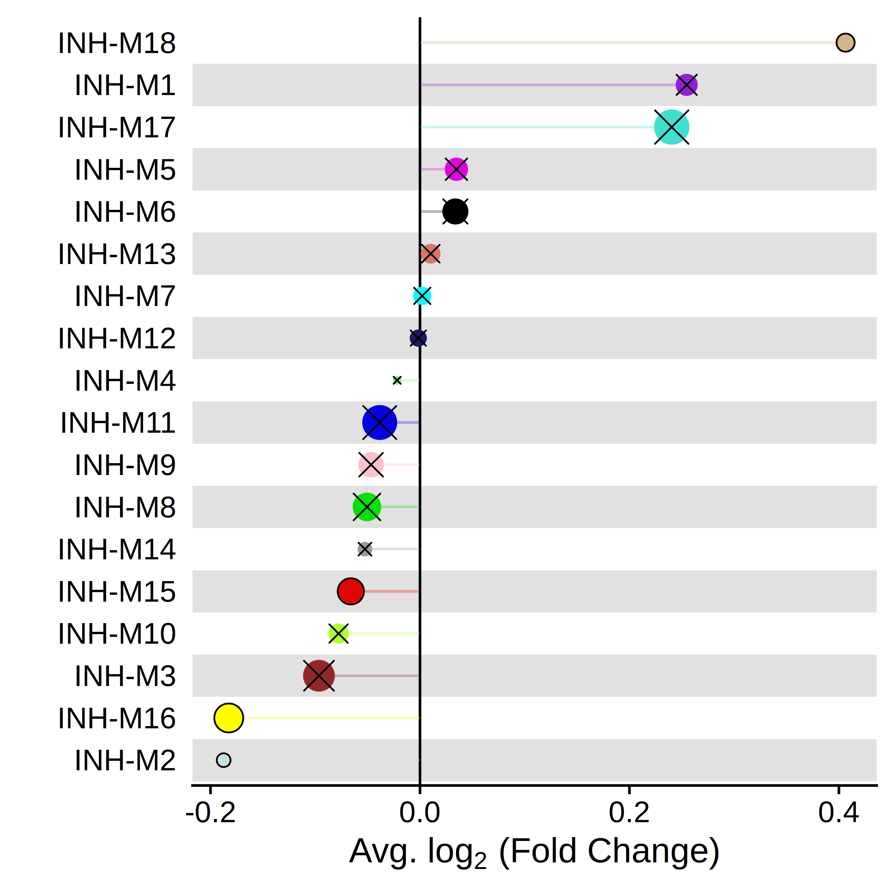
该图显示了每个模块的fold change,每个点的大小对应于该模块中基因的数量, X表示该点没有达到统计显著性。
对于PlotDMEsLollipop,如果我们在DMEs的data frame中有其他自定义列,我们可以使用group.by为一个比较组或用于绘图的比较组列表提供列名和比较参数。例如:
1 | |
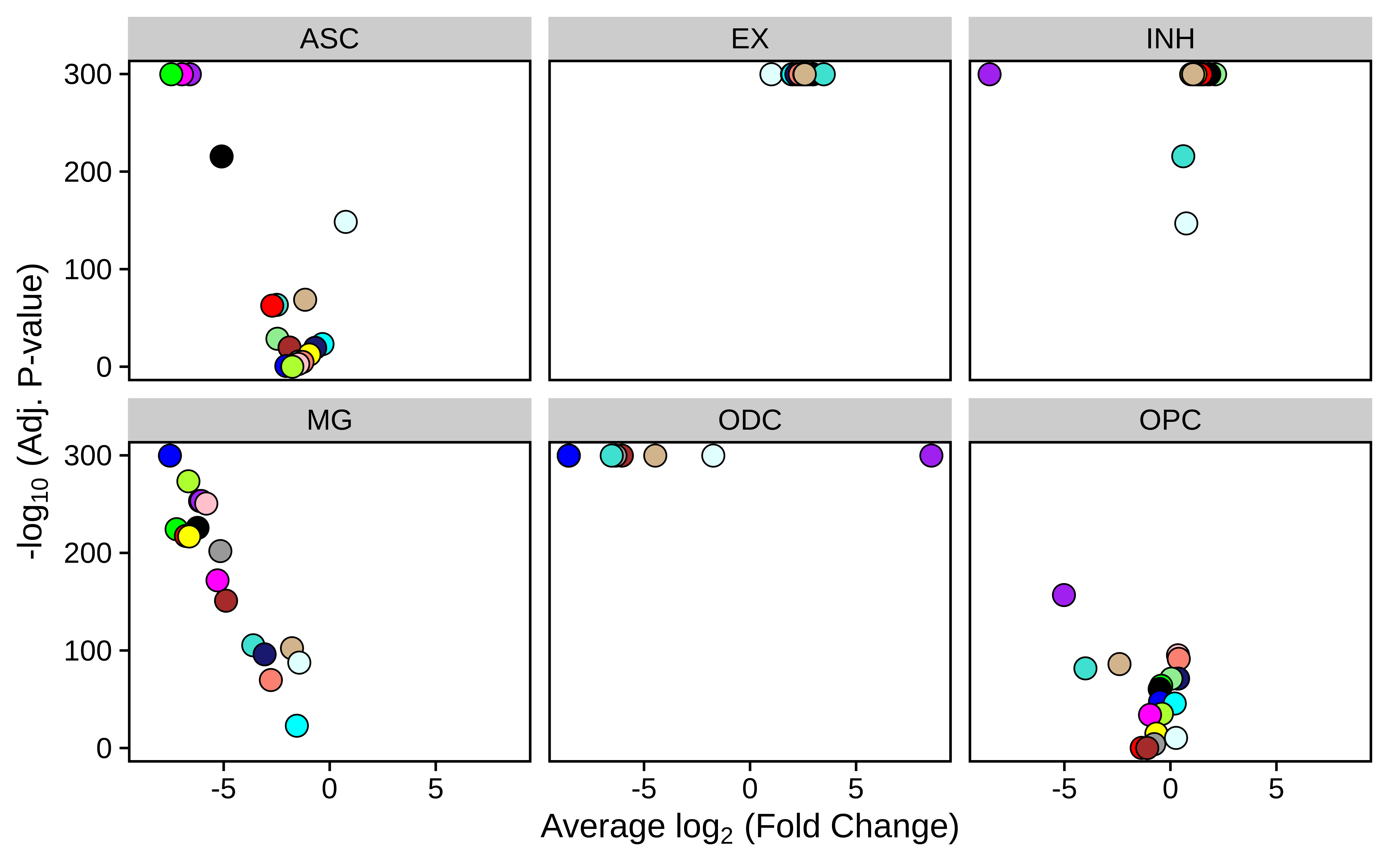
使用函数PlotDMEsVolcano将结果可视化。
使用PlotDMEsVolcano来制作火山图,以显示fold change和显著性水平。
1 | |
一对多的DME分析
与Seurat函数FindAllMarkers类似,在指定要分组cell的列时,可以使用函数FindAllDMEs执行单对全的DME测试。我们在这里分组。通过每个细胞类型进行一对一的测试。
1 | |
绘图
1 | |
8.模块特征相关性分析
计算相关性
使用函数ModuleTraitCorrelation将选定的变量与模块特征基因相关联。该函数计算指定分组的相关性,因为我们可以预期某些变量可能与分组中的某些模块相关,但与其他单元组中的模块无关。在这里要注意输入变量的数据类型:
可以使用的变量包括:
- 数值变量
- 只有 2 个类别的分类变量,例如“CONTROL”和“CASE”。
- 具有levels的分类变量,数据格式需要为因子型数据。例如,您可能有一个“疾病阶段”类别,按“健康”、“阶段 1”、“阶段 2”、“阶段 3”等排序。
不能使用的变量:
具有两个以上无排序的分类变量。比如“sampleid”变量,由于这个变量的排序不一定有生物学意义,因此这样的变量不适合模块性状相关分析。再举个例子:假设有一个由三种转基因小鼠品系和一种对照小鼠组成的数据集。由于没法对这个分类进行排序,在运行相关性之前,必须将分类变量转换为数字,因此最终会得到完全没有生物学意义的相关性。在这种情况下,应该分别在对照和每个转基因小鼠品系之间建立成对的相关性比较。
1 | |
对于使用的任何分类变量,使用ModuleTraitCorrelation函数都会打印出一条警告消息,可忽视该警告,警告只是为了确保输入的分类变量有生物学意义。
检查输出
mt_cor是一个列表;cor保存相关结果,pval保存相关 p 值,fdr保存 FDR 校正的 p 值。
1 | |
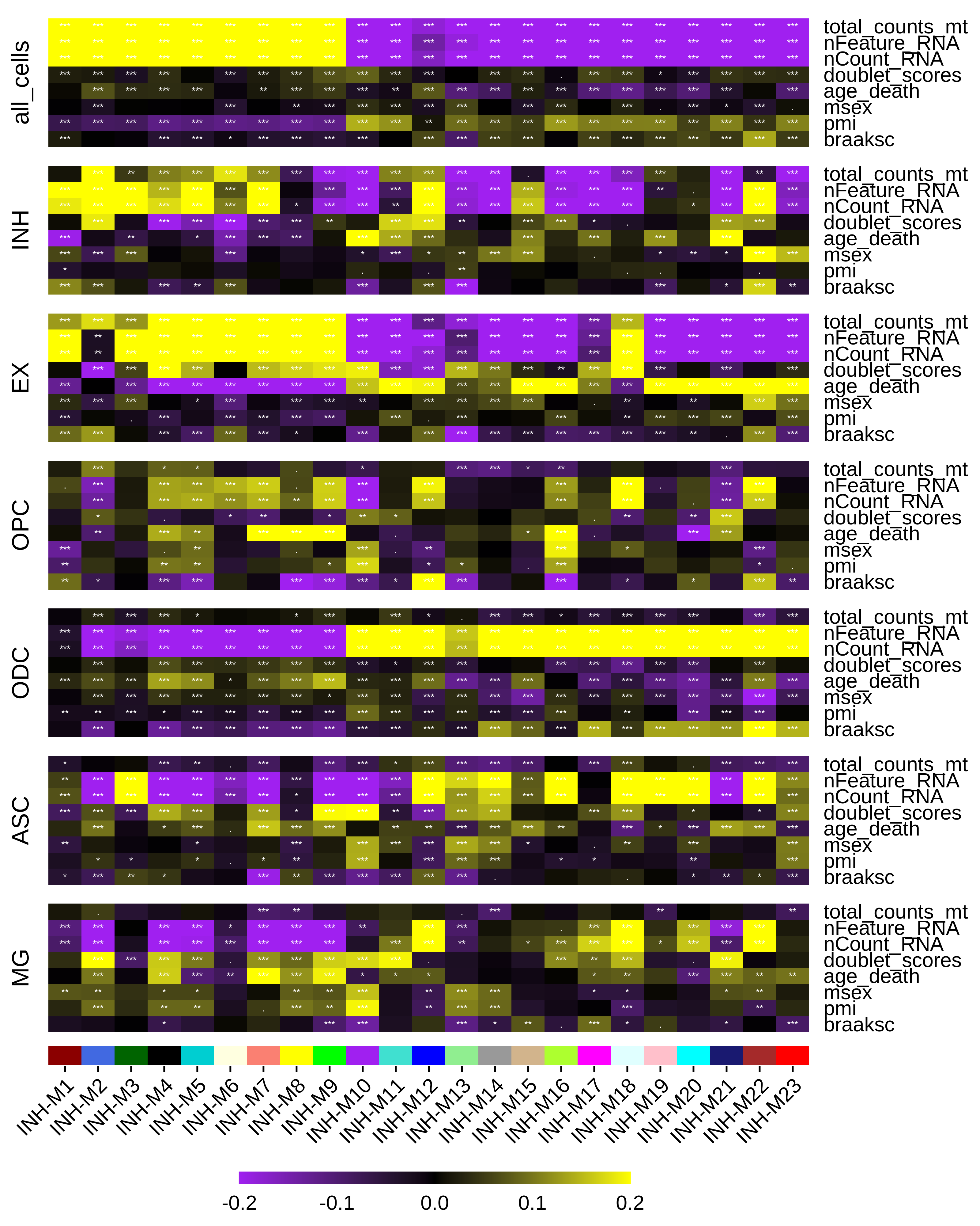
绘制相关热图
使用PlotModuleTraitCorrelation函数绘制相关性分析的结果。该函数为每个相关性矩阵创建一个单独的热图,然后进行拼图。
1 | |
hdWGCNA与WGCNA R包比较
- 使用WGCNA分析scRNA数据时,需要提取表达量矩阵进行分析。hdWGCNA可直接对接Seurat R包,直接基于Seurat结果进行下游分析:每个clusters随机抽取20%的细胞,可以选择使用全部的基因或者仅使用seurat挑选出来的高变基因,以及不同的降维方式和维度数,用于共表达模块的WGCNA检测,选取软阈值。中间部分与WGCNA无区别。最后,在单细胞空间中计算不同模块的平均表达式,并绘制降维图。生成所有模块的图表示,并可选择进行对应的GO富集分析。
- 基于metacells重新进行normalize后的数据进行分析,考虑到单细胞矩阵稀疏的特点,增加了数据的稳健性。
- 下游可视化形式更加丰富,除了WGCNA经典的模块与性状相关性热图,模块识别聚类树图等,增加了结合Seurat进行可视化,网络分析,差异模块特征基因(类似差异分析)分析,富集分析(图片有点丑),将生成的模块信息投影到其他数据集(可以将单细胞数据生成的模块信息投影到ATAC-seq,空转或者其他物种的单细胞数据集中)的内容。
- hdWGCNA中的TOM图可视化需要手动实现。
- hdWGCNA主要集中在对模块特征基因的展示,并以umap形式提供模块中全部基因的展示(与WGCNA生成的聚类图箱线图和柱状图相比,在细胞数和基因数较多时可视化方式更友好)。
hdWGCNA耗时统计
demo数据 36601基因,36671细胞
- SetUpForWGCN初始化设置耗时:1.690009 mins
- Meta细胞构建: 6.070287 mins
- SetDatExpr运行时间: 0.6600406 secs
- 软阈值选择: 50.69805 secs
- 构建共表达网络耗时:5.24069 mins
- 模块特征基因: 1.20085 hours
复习关键名词
- ME:通过对包含每个模块的基因表达矩阵执行(PCA)来计算获得的“伪基因”。每个PCA矩阵的第一个PC是MEs。
- kME: 是根据MEs的连通性的排名,排名越高,就证明这个基因是共表达网络中高度连接的成员,主要用于筛选hub-gene.
- hME: 对MEs使用Harmony对sampleid矫正后获得的值。在基础可视化部分默认用到。